next year's y = rate * y * (1 - y)The "(1-y)" term is the limiting factor preventing a harrowing fish population explosion. But the model has become more abstract, because the population (y) is now measured from zero (no fish) to one (the largest possible number of fish). The equation is called the logistic difference equation.
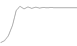
A graph of this equation, with an initial population (y) of 0.02 and a growth rate of 2.7 gives the following graph over time:
